2. Tutorial
2.1. Follow along
Code for all the examples is located in your PYTHONPATH/Lib/site-packages/eonr/examples folder. With that said, you should be able to make use of EONR by following and executing the commands in this tutorial using either the sample data provided or substituting in your own data.
You will find the following code included in the tutorial.py or tutorial.ipynb (for Jupyter notebooks) files in your PYTHONPATH/Lib/site-packages/eonr/examples folder - feel free to load that into your Python IDE to follow along.
2.2. Load modules
After installation, load Pandas and the EONR module in a Python interpreter:
[1]:
import os
import pandas as pd
import eonr
print('EONR version: {0}'.format(eonr.__version__))
EONR version: 0.2.0
2.3. Load the data
EONR uses Pandas dataframes to access and manipulate the experimental data.
[2]:
df_data = pd.read_csv(os.path.join('data', 'minnesota_2012.csv'))
df_data
[2]:
| year | location | plot | trt | rep | time_n | rate_n_applied_kgha | yld_grain_dry_kgha | nup_total_kgha | soil_plus_fert_n_kgha | |
|---|---|---|---|---|---|---|---|---|---|---|
| 0 | 2012 | Minnesota | 101 | 8 | 1 | Pre | 235.3785 | 12410.916200 | 198.759898 | 284.69590 |
| 1 | 2012 | Minnesota | 102 | 3 | 1 | Pre | 67.2510 | 10627.946000 | 147.971755 | 116.56840 |
| 2 | 2012 | Minnesota | 103 | 1 | 1 | Pre | 0.0000 | 7428.081218 | 98.769392 | 38.10890 |
| 3 | 2012 | Minnesota | 104 | 2 | 1 | Pre | 33.6255 | 9202.953180 | 111.440210 | 71.73440 |
| 4 | 2012 | Minnesota | 105 | 4 | 2 | Pre | 100.8765 | 10841.127180 | 142.663887 | 154.67730 |
| 5 | 2012 | Minnesota | 106 | 7 | 2 | Pre | 201.7530 | 10646.649330 | 178.802092 | 255.55380 |
| 6 | 2012 | Minnesota | 107 | 6 | 2 | Pre | 168.1275 | 12367.436000 | 186.053531 | 201.75300 |
| 7 | 2012 | Minnesota | 108 | 5 | 2 | Pre | 134.5020 | 13366.361700 | 196.737290 | 168.12750 |
| 8 | 2012 | Minnesota | 201 | 7 | 1 | Pre | 201.7530 | 14232.053480 | 228.775204 | 251.07040 |
| 9 | 2012 | Minnesota | 202 | 5 | 1 | Pre | 134.5020 | 14384.824980 | 226.006218 | 183.81940 |
| 10 | 2012 | Minnesota | 203 | 6 | 1 | Pre | 168.1275 | 13592.219290 | 182.423028 | 206.23640 |
| 11 | 2012 | Minnesota | 204 | 4 | 1 | Pre | 100.8765 | 14091.078390 | 187.745096 | 138.98540 |
| 12 | 2012 | Minnesota | 205 | 3 | 2 | Pre | 67.2510 | 10739.981390 | 133.470950 | 121.05180 |
| 13 | 2012 | Minnesota | 206 | 1 | 2 | Pre | 0.0000 | 8375.090921 | 109.460245 | 53.80080 |
| 14 | 2012 | Minnesota | 207 | 8 | 2 | Pre | 235.3785 | 13797.485850 | 195.932161 | 269.00400 |
| 15 | 2012 | Minnesota | 208 | 2 | 2 | Pre | 33.6255 | 9713.487469 | 113.903035 | 67.25100 |
| 16 | 2012 | Minnesota | 301 | 3 | 3 | Pre | 67.2510 | 12579.012170 | 180.812783 | 106.48075 |
| 17 | 2012 | Minnesota | 302 | 7 | 3 | Pre | 201.7530 | 13604.571780 | 208.724988 | 240.98275 |
| 18 | 2012 | Minnesota | 303 | 2 | 3 | Pre | 33.6255 | 10185.959390 | 121.505528 | 68.37185 |
| 19 | 2012 | Minnesota | 304 | 6 | 3 | Pre | 168.1275 | 14305.321460 | 204.391319 | 202.87385 |
| 20 | 2012 | Minnesota | 305 | 8 | 4 | Pre | 235.3785 | 13929.592020 | 186.775288 | 267.88315 |
| 21 | 2012 | Minnesota | 306 | 4 | 4 | Pre | 100.8765 | 10975.799250 | 147.057081 | 133.38115 |
| 22 | 2012 | Minnesota | 307 | 5 | 4 | Pre | 134.5020 | 11338.070290 | 148.348790 | 162.52325 |
| 23 | 2012 | Minnesota | 308 | 1 | 4 | Pre | 0.0000 | 5821.373521 | 68.791363 | 28.02125 |
| 24 | 2012 | Minnesota | 401 | 5 | 3 | Pre | 134.5020 | 13755.002370 | 198.844611 | 173.73175 |
| 25 | 2012 | Minnesota | 402 | 1 | 3 | Pre | 0.0000 | 9077.628329 | 122.207140 | 39.22975 |
| 26 | 2012 | Minnesota | 403 | 4 | 3 | Pre | 100.8765 | 13760.323240 | 181.734857 | 135.62285 |
| 27 | 2012 | Minnesota | 404 | 8 | 3 | Pre | 235.3785 | 14896.886860 | 227.454749 | 270.12485 |
| 28 | 2012 | Minnesota | 405 | 2 | 4 | Pre | 33.6255 | 10551.466010 | 144.282839 | 66.13015 |
| 29 | 2012 | Minnesota | 406 | 6 | 4 | Pre | 168.1275 | 15621.406530 | 227.056199 | 200.63215 |
| 30 | 2012 | Minnesota | 407 | 3 | 4 | Pre | 67.2510 | 10950.450720 | 146.628851 | 95.27225 |
| 31 | 2012 | Minnesota | 408 | 7 | 4 | Pre | 201.7530 | 13838.222530 | 210.340625 | 229.77425 |
2.4. Set column names (pre-init)
The table containing the experimental data must have a minimum of two columns:
Nitrogen fertilizer rate
Grain yield
EONR accepts custom column names. Just be sure to set them by either using EONR.set_column_names() or by passing them to EONR.calculate_eonr(). We will declare the names of the these two columns as they exist in the Pandas dataframe so they can be passed to EONR later:
[3]:
col_n_app = 'rate_n_applied_kgha'
col_yld = 'yld_grain_dry_kgha'
Each row of data in our dataframe should correspond to a nitrogen rate treatment plot. It is common to have several other columns describing each treatment plot (e.g., year, location, replication, nitrogen timing, etc.). These aren’t necessary, but EONR will try pull information from “year”, “location”, and “nitrogen timing” for labeling the plots that are generated (as you’ll see towards the end of this tutorial).
2.5. Set units
Although optional, it is good practice to declare units so we don’t get confused:
[4]:
unit_currency = '$'
unit_fert = 'kg'
unit_grain = 'kg'
unit_area = 'ha'
These unit variables are only used for plotting (titles and axes labels), and they are not actually used for any computations. Because the initial parameter guess is critically important for fitting the model(s), there is logic built in that adjusts this intitial guess based on the units provided here.
2.6. Set economic conditions
EONR computes the Economic Optimum Nitrogen Rate for any economic scenario that we define. All that is required is to declare the cost of the nitrogen fertilizer (per unit, as defined above) and the price of grain (also per unit). Note that the cost of nitrogen fertilizer can be set to zero, and the Agronomic Optimum Nitrogen Rate will be computed.
[5]:
cost_n_fert = 0.88  # in USD per kg nitrogen
price_grain = 0.157  # in USD per kg grain
2.7. Initialize EONR
At this point, we can initialize an instance of EONR.
Before doing so, we may want to set the base directory. EONR.base_dir is the default location for saving plots and data processed by EONR. If EONR.base_dir is not set, it will be set to be a folder named “eonr_tutorial” in the current working directory during the intitialization (to see your current working directory, type os.getcwd()). If you do not wish to use this as your current working directory, it can be passed to the EONR instance using the
base_dir keyword.
For demonstration purposes, we will set EONR.base_dir to what would be the default folder if nothing were passed to the base_dir keyword –> that is, we will choose a folder named “eonr_advanced_tutorial” in the current working directory (EONR will create the directory if it does not exist).
And finally, to create an instance of EONR, pass the appropriate variables to EONR():
[6]:
import os
base_dir = os.path.join(os.getcwd(), 'eonr_tutorial')

my_eonr = eonr.EONR(cost_n_fert=cost_n_fert,
                    price_grain=price_grain,
                    col_n_app=col_n_app,
                    col_yld=col_yld,
                    unit_currency=unit_currency,
                    unit_grain=unit_grain,
                    unit_fert=unit_fert,
                    unit_area=unit_area,
                    model=None,
                    base_dir=base_dir)
Notice the model keywork argument was set to None (default=’quad_plateau’). This keyword is used to define which model to use to fit the experimental data. If None, EONR will try all supported models (i.e., as of v. 0.2.0, both ‘quad_plateau’ and ‘quadratic’ models are supported), and use the model that fits the data best as determined by the highest \(\text{r}^2\).
2.8. Calculate the EONR
With my_eonr initialized as an instance of EONR, we can now calculate the economic optimum nitrogen rate by calling the calculate_eonr() method and passing the dataframe with the loaded data:
[7]:
my_eonr.calculate_eonr(df_data)
Computing EONR for Minnesota 2012 Pre
Cost of N fertilizer: $0.88 per kg
Price grain: $0.16 per kg
Fixed costs: $0.00 per ha
Checking quadratic and quadric-plateau models for best fit..
Quadratic model r^2: 0.72
Quadratic-plateau model r^2: 0.73
Using the quadratic-plateau model..
Economic optimum N rate (EONR): 162.3 kg per ha [130.5, 207.8] (90.0% confidence)
Maximum return to N (MRTN): $767.93 per ha
It may take a few seconds to run, but it will take much longer if you choose to compute the bootstrap confidence intervals in addition to the profile-likelihood confidence intervals. Please see the Advanced tutorial describing how to compute the bootstrap CIs (EONR does not run the bootstrap CIs by default).
And that’s it! The economic optimum for this dataset and economic scenario was 162 kg nitrogen per ha (with 90% confidence bounds at 131 and 208 kg per ha) and resulted in a maximum net return of nearly $770 per ha.
Notice the \(\text{r}^2\) for the quadratic-plateau model was greater than that of the quadratic model, so the quadratic-plateau model was used (the model used is recorded in EONR.df_results and will be displayed in the plot legend - see below).
2.9. Plotting the EONR
This is great, but of course it’d be useful to see our data and results plotted. Do this by calling the plot_eonr() module and (optionally) passing the minimum/maximum values for each axis:
[8]:
my_eonr.plot_eonr(x_min=-5, x_max=300, y_min=-100, y_max=1400)
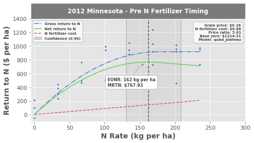
The blue points are experimental data (yield value in \$ per ha as a function of nitrogen rate)
The blue line is the best-fit quadratic-plateau model representing gross return to nitrogen
The red line is the cost of nitrogen fertilizer
The green line is the difference between the two and represents the net return to nitrogen
The green point is the Economic Optimum Nitrogen Rate (EONR)
The transparent grey box surrounding the EONR/MRTN (green point) illustrates the 90% confidence intervals
The EONR is the point on the x-axis where the net return curve (green) reaches the maximum return. The return to nitrogen at the EONR is the Maximum Return to Nitrogen (MRTN), indicating the profit that is earned at the economic optimum nitrogen rate.
Notice the economic scenario (i.e., grain price, nitrogen fertilizer cost, etc.) and the “Base zero” values in the upper right corner describing the assumptions of EONR calculatioon. Base zero refers to the initial y-intercept of the gross return model (this setting can be turned on/off by setting EONR.base_zero to True or False. See the Advanced tutorial and the API for more information.
2.10. Accesing complete results
All results (e.g., EONR, MRTN, \(\text{r}^2\) and root mean squared errors from best-fit models, confidence intervals, etc.) are stored in the EONR.df_results dataframe:
[9]:
my_eonr.df_results
[9]:
| price_grain | cost_n_fert | cost_n_social | costs_fixed | price_ratio | unit_price_grain | unit_cost_n | location | year | time_n | ... | mrtn | grtn_r2_adj | grtn_rmse | grtn_max_y | grtn_crit_x | grtn_y_int | scn_lin_r2 | scn_lin_rmse | scn_exp_r2 | scn_exp_rmse | |
|---|---|---|---|---|---|---|---|---|---|---|---|---|---|---|---|---|---|---|---|---|---|
| 0 | 0.157 | 0.88 | 0.0 | 0.0 | 5.605096 | $ per ha | $ per kg | Minnesota | 2012 | Pre | ... | 767.930477 | 0.728926 | 181.225993 | 917.43358 | 177.439985 | 0.002964 | None | None | None | None |
1 rows × 33 columns
See the Advanced tutorial for a description of every column.
2.11. Visualizing all confidence intervals
By default, the confidence intervals (CIs) are calculated at many alpha levels. Noting that \(\text{CI} = 1-\alpha\), let’s plot the Wald CIs and profile-likelihood CIs for a range of \(\alpha\) values.
EONR.plot_modify_size() can be called to make basic adjustments to the figure size. Because EONR.fig_tau.fig is a Matplotlib figure object, you’ll be able to make any customizations within the Matplotlib API as well.
[10]:
my_eonr.plot_tau()
my_eonr.fig_tau = my_eonr.plot_modify_size(fig=my_eonr.fig_tau.fig, plotsize_x=5, plotsize_y=4.0)
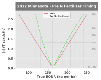
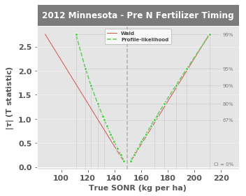
This plot shows the lower and upper confidence intervals of the True EONR (True EONR refers to the actual EONR value, which is not actually known due to uncertainty in the dataset). At 0% confidence, the True EONR is the maximum likelihood value, but as we increase the confidence level from 67%, 80%, 90%, 95%, and 99%, the statistical range of the True EONR widens.
In general, the profile-likelihood CIs are considered the most accurate of the three methods because they reflect the actual, often asymmetric, uncertainty in a parameter estimate Cook & Weisberg, 1990.
2.12. Accessing complete CI results
All data relating to the calculation of the CIs are saved in the EONR.df_ci dataframe:
[11]:
my_eonr.df_ci
[11]:
| run_n | location | year | time_n | price_grain | cost_n_fert | cost_n_social | price_ratio | f_stat | t_stat | level | wald_l | wald_u | pl_l | pl_u | boot_l | boot_u | opt_method_l | opt_method_u | |
|---|---|---|---|---|---|---|---|---|---|---|---|---|---|---|---|---|---|---|---|
| 0 | 1 | Minnesota | 2012 | Pre | 0.157 | 0.88 | 0.0 | 5.605096 | 0.000000 | 0.000000 | 0.000 | NaN | NaN | NaN | NaN | NaN | NaN | N/A | N/A |
| 1 | 1 | Minnesota | 2012 | Pre | 0.157 | 0.88 | 0.0 | 5.605096 | 0.016070 | 0.126767 | 0.100 | 158.247550 | 166.432039 | 159.432270 | 165.322890 | NaN | NaN | Nelder-Mead | Nelder-Mead |
| 2 | 1 | Minnesota | 2012 | Pre | 0.157 | 0.88 | 0.0 | 5.605096 | 0.065374 | 0.255684 | 0.200 | 154.085886 | 170.593703 | 156.557488 | 168.432973 | NaN | NaN | Nelder-Mead | Nelder-Mead |
| 3 | 1 | Minnesota | 2012 | Pre | 0.157 | 0.88 | 0.0 | 5.605096 | 0.151446 | 0.389161 | 0.300 | 149.777004 | 174.902584 | 153.670496 | 171.730580 | NaN | NaN | Nelder-Mead | Nelder-Mead |
| 4 | 1 | Minnesota | 2012 | Pre | 0.157 | 0.88 | 0.0 | 5.605096 | 0.281127 | 0.530214 | 0.400 | 145.223559 | 179.456029 | 150.721517 | 175.297880 | NaN | NaN | Nelder-Mead | Nelder-Mead |
| 5 | 1 | Minnesota | 2012 | Pre | 0.157 | 0.88 | 0.0 | 5.605096 | 0.466549 | 0.683044 | 0.500 | 140.289960 | 184.389628 | 147.647498 | 179.255088 | NaN | NaN | Nelder-Mead | Nelder-Mead |
| 6 | 1 | Minnesota | 2012 | Pre | 0.157 | 0.88 | 0.0 | 5.605096 | 0.729644 | 0.854192 | 0.600 | 134.765004 | 189.914585 | 144.357366 | 183.796319 | NaN | NaN | Nelder-Mead | Nelder-Mead |
| 7 | 1 | Minnesota | 2012 | Pre | 0.157 | 0.88 | 0.0 | 5.605096 | 0.969292 | 0.984526 | 0.667 | 130.557584 | 194.122004 | 141.960754 | 187.330059 | NaN | NaN | Nelder-Mead | Nelder-Mead |
| 8 | 1 | Minnesota | 2012 | Pre | 0.157 | 0.88 | 0.0 | 5.605096 | 1.113663 | 1.055302 | 0.700 | 128.272818 | 196.406771 | 140.698855 | 189.275802 | NaN | NaN | Nelder-Mead | Nelder-Mead |
| 9 | 1 | Minnesota | 2012 | Pre | 0.157 | 0.88 | 0.0 | 5.605096 | 1.719858 | 1.311434 | 0.800 | 120.004454 | 204.675134 | 136.361782 | 196.472716 | NaN | NaN | Nelder-Mead | Nelder-Mead |
| 10 | 1 | Minnesota | 2012 | Pre | 0.157 | 0.88 | 0.0 | 5.605096 | 2.887033 | 1.699127 | 0.900 | 107.489043 | 217.190545 | 130.457577 | 207.827070 | NaN | NaN | Nelder-Mead | Nelder-Mead |
| 11 | 1 | Minnesota | 2012 | Pre | 0.157 | 0.88 | 0.0 | 5.605096 | 4.182964 | 2.045230 | 0.950 | 96.316254 | 228.363335 | 125.804436 | 218.441868 | NaN | NaN | Nelder-Mead | Nelder-Mead |
| 12 | 1 | Minnesota | 2012 | Pre | 0.157 | 0.88 | 0.0 | 5.605096 | 7.597663 | 2.756386 | 0.990 | 73.358903 | 251.320685 | 117.769597 | 241.793290 | NaN | NaN | Nelder-Mead | Nelder-Mead |
2.13. Adjusting the economic scenario
These results were calculated for a specific economic scenario, but the cost of fertilizer and price of grain can be adjusted to run EONR for another economic scenario. Just adjust the economic scenario by passing any of:
cost_n_fertprice_graincost_n_social
to EONR.update_econ():
[12]:
cost_n_fert = 1.32  # adjusted from $0.88 per kg nitrogen
my_eonr.update_econ(cost_n_fert=cost_n_fert)
2.14. Environmental observations
You’ll notice above that we can pass the cost_n_social variable to EONR.update_econ(). This is becuase EONR will calculate the Socially Optimum Nitrogen Rate (SONR) if certain environmental data are available. For more information about the SONR, refer to the Background chapter.
In the same way that cost_n_fert was adjusted in the previous code, cost_n_social will be set (for the first time):
[13]:
cost_n_social = 1.10 # in USD per kg nitrogen
my_eonr.update_econ(cost_n_social=cost_n_social)
2.15. Calculate mineralization
You may have noticed that the loaded data for this tutorial contains columns for nitrogen uptake (“nup_total_kgha”) and available nitrogen (“soil_plus_fert_n_kgha”). This data can be used to calculate the approximate net mineralization for the zero rate, which can be assumed to consistent across all rates. Total crop available nitrogen can then be assumed to be the sum of fertilizer, soil, and net mineralized nitrogen. We can then calculate the SONR as long as the column names are correctly set.
The column names were set for nitrogen fertilizer rate (col_n_app) and grain yield (col_yld) during the initialization of EONR, but they haven’t been set for the nitrogen uptake or available nitrogen columns. This can be done (even after initilization of EONR) using EONR.set_column_names():
[14]:
def calc_mineralization(df_data, units_fert='kgha'):
    '''
    Calculates mineralization and adds "crop_available_n" to df
    '''
    df_trt0 = df_data[df_data['rate_n_applied_kgha']==0].copy()
    df_trt0['mineralize_n'] = (df_trt0['nup_total_kgha'] -
                               df_trt0['soil_plus_fert_n_kgha'])
    trt0_mineralize = df_trt0['mineralize_n'].mean()
    crop_n_label = 'crop_n_available_' + units_fert
    df_data[crop_n_label] = df_data['soil_plus_fert_n_kgha'] + trt0_mineralize
    return df_data

df_data = calc_mineralization(df_data)

col_crop_nup = 'nup_total_kgha'
col_n_avail = 'crop_n_available_kgha'

my_eonr.set_column_names(col_crop_nup=col_crop_nup,
                         col_n_avail=col_n_avail)
EONR simply subtracts end of season total nitrogen uptake from available nitrogen to get net crop nitrogen use, which is subsequently used to calculate the SONR.
2.16. Run EONR for the socially optimum rate
Then simply run EONR.calculate_eonr() again to calculate the SONR for the updated economic scenario:
[15]:
my_eonr.calculate_eonr(df_data)
Computing SONR for Minnesota 2012 Pre
Cost of N fertilizer: $1.32 per kg
Price grain: $0.16 per kg
Fixed costs: $0.00 per ha
Social cost of N: $1.10 per kg
Checking quadratic and quadric-plateau models for best fit..
Quadratic model r^2: 0.72
Quadratic-plateau model r^2: 0.73
Using the quadratic-plateau model..
Socially optimum N rate (SONR): 149.6 kg per ha [122.4, 186.3] (90.0% confidence)
Maximum return to N (MRTN): $684.60 per ha
The new results are appended to the EONR.df_results dataframe:
[16]:
my_eonr.df_results
[16]:
| price_grain | cost_n_fert | cost_n_social | costs_fixed | price_ratio | unit_price_grain | unit_cost_n | location | year | time_n | ... | mrtn | grtn_r2_adj | grtn_rmse | grtn_max_y | grtn_crit_x | grtn_y_int | scn_lin_r2 | scn_lin_rmse | scn_exp_r2 | scn_exp_rmse | |
|---|---|---|---|---|---|---|---|---|---|---|---|---|---|---|---|---|---|---|---|---|---|
| 0 | 0.157 | 0.88 | 0.0 | 0.0 | 5.605096 | $ per ha | $ per kg | Minnesota | 2012 | Pre | ... | 767.930477 | 0.728926 | 181.225993 | 917.43358 | 177.439985 | 0.002964 | None | None | None | None |
| 1 | 0.157 | 1.32 | 1.1 | 0.0 | 15.414013 | $ per ha | $ per kg | Minnesota | 2012 | Pre | ... | 684.596933 | 0.728926 | 181.225993 | 917.43358 | 177.439985 | 0.002964 | 0.777106 | 139.314 | 0.836099 | 21.1184 |
2 rows × 33 columns
EONR.plot_eonr() and EONR.plot_tau() can be called again to plot the new results:
[17]:
my_eonr.plot_eonr(x_min=-5, x_max=300, y_min=-200, y_max=1400)
my_eonr.plot_tau()
fig_tau = my_eonr.plot_modify_size(fig=my_eonr.fig_tau.fig, plotsize_x=5, plotsize_y=4.0)
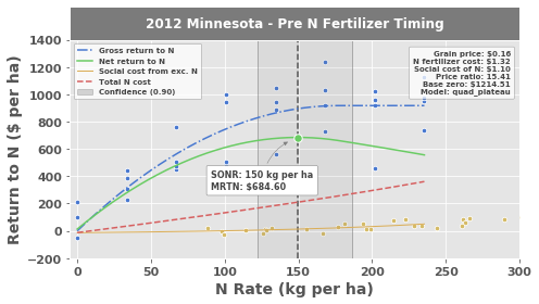
Notice the added data in the nitrogen response plot:
The gold points represent net crop nitrogen use (expressed as a \$ amount based on the value set for
cost_n_social)The gold line is the best-fit exponential model representing net crop nitrogen use (
EONRfits both a linear and exponential model for this, then uses whichever has a higher \(\text{r}^2\))
2.17. Saving the data
The results generated by EONR can be saved to the EONR.base_dir using the Pandas df.to_csv() function. A folder will be created in the base_dir whose name is determined by the current economic scenario of my_eonr (in this case “social_154_1100”, corresponding to cost_n_social > 0, price_ratio = 15.4, and cost_n_social = 1.10 for “social”, “154”, and “1100” in the folder name, respectively):
[18]:
print(my_eonr.base_dir)

my_eonr.df_results.to_csv(os.path.join(os.path.split(my_eonr.base_dir)[0], 'tutorial_results.csv'), index=False)
my_eonr.df_ci.to_csv(os.path.join(os.path.split(my_eonr.base_dir)[0], 'tutorial_ci.csv'), index=False)
F:\nigo0024\Documents\GitHub\eonr\docs\source\eonr_tutorial\social_154_1100
Upon generating figures using EONR.plot_eonr() or EONR.plot_tau(), the matplotlib figures are stored to the EONR class. They can be saved to file by using EONR.plot_save():
[19]:
fname_eonr_plot = 'eonr_mn2012_pre.png'
fname_tau_plot = 'tau_mn2012_pre.png'

my_eonr.plot_save(fname=fname_eonr_plot, fig=my_eonr.fig_eonr)
my_eonr.plot_save(fname=fname_tau_plot, fig=my_eonr.fig_tau)