3. Advanced Tutorial
3.1. Follow along
Code for all the examples is located in your PYTHONPATH/Lib/site-packages/eonr/examples folder. With that said, you should be able to make use of EONR by following and executing the commands in this tutorial using either the sample data provided or substituting in your own data.
You will find the following code included in the advanced_tutorial.py or advanced_tutorial.ipynb (for Jupyter notebooks) files in your PYTHONPATH/Lib/site-packages/eonr/examples folder - feel free to load that into your Python IDE to follow along.
3.2. Calculate EONR for several economic scenarios
In this tutorial, we will run EONR.calculate_eonr() in a loop, adjusting the economic scenario prior to each run.
3.3. Load modules
Load pandas and EONR:
[1]:
import os
import pandas as pd
import eonr
print('EONR version: {0}'.format(eonr.__version__))
EONR version: 0.2.0
3.4. Load the data
EONR uses Pandas dataframes to access and manipulate the experimental data.
[2]:
df_data = pd.read_csv(os.path.join('data', 'minnesota_2012.csv'))
df_data
[2]:
| year | location | plot | trt | rep | time_n | rate_n_applied_kgha | yld_grain_dry_kgha | nup_total_kgha | soil_plus_fert_n_kgha | |
|---|---|---|---|---|---|---|---|---|---|---|
| 0 | 2012 | Minnesota | 101 | 8 | 1 | Pre | 235.3785 | 12410.916200 | 198.759898 | 284.69590 |
| 1 | 2012 | Minnesota | 102 | 3 | 1 | Pre | 67.2510 | 10627.946000 | 147.971755 | 116.56840 |
| 2 | 2012 | Minnesota | 103 | 1 | 1 | Pre | 0.0000 | 7428.081218 | 98.769392 | 38.10890 |
| 3 | 2012 | Minnesota | 104 | 2 | 1 | Pre | 33.6255 | 9202.953180 | 111.440210 | 71.73440 |
| 4 | 2012 | Minnesota | 105 | 4 | 2 | Pre | 100.8765 | 10841.127180 | 142.663887 | 154.67730 |
| 5 | 2012 | Minnesota | 106 | 7 | 2 | Pre | 201.7530 | 10646.649330 | 178.802092 | 255.55380 |
| 6 | 2012 | Minnesota | 107 | 6 | 2 | Pre | 168.1275 | 12367.436000 | 186.053531 | 201.75300 |
| 7 | 2012 | Minnesota | 108 | 5 | 2 | Pre | 134.5020 | 13366.361700 | 196.737290 | 168.12750 |
| 8 | 2012 | Minnesota | 201 | 7 | 1 | Pre | 201.7530 | 14232.053480 | 228.775204 | 251.07040 |
| 9 | 2012 | Minnesota | 202 | 5 | 1 | Pre | 134.5020 | 14384.824980 | 226.006218 | 183.81940 |
| 10 | 2012 | Minnesota | 203 | 6 | 1 | Pre | 168.1275 | 13592.219290 | 182.423028 | 206.23640 |
| 11 | 2012 | Minnesota | 204 | 4 | 1 | Pre | 100.8765 | 14091.078390 | 187.745096 | 138.98540 |
| 12 | 2012 | Minnesota | 205 | 3 | 2 | Pre | 67.2510 | 10739.981390 | 133.470950 | 121.05180 |
| 13 | 2012 | Minnesota | 206 | 1 | 2 | Pre | 0.0000 | 8375.090921 | 109.460245 | 53.80080 |
| 14 | 2012 | Minnesota | 207 | 8 | 2 | Pre | 235.3785 | 13797.485850 | 195.932161 | 269.00400 |
| 15 | 2012 | Minnesota | 208 | 2 | 2 | Pre | 33.6255 | 9713.487469 | 113.903035 | 67.25100 |
| 16 | 2012 | Minnesota | 301 | 3 | 3 | Pre | 67.2510 | 12579.012170 | 180.812783 | 106.48075 |
| 17 | 2012 | Minnesota | 302 | 7 | 3 | Pre | 201.7530 | 13604.571780 | 208.724988 | 240.98275 |
| 18 | 2012 | Minnesota | 303 | 2 | 3 | Pre | 33.6255 | 10185.959390 | 121.505528 | 68.37185 |
| 19 | 2012 | Minnesota | 304 | 6 | 3 | Pre | 168.1275 | 14305.321460 | 204.391319 | 202.87385 |
| 20 | 2012 | Minnesota | 305 | 8 | 4 | Pre | 235.3785 | 13929.592020 | 186.775288 | 267.88315 |
| 21 | 2012 | Minnesota | 306 | 4 | 4 | Pre | 100.8765 | 10975.799250 | 147.057081 | 133.38115 |
| 22 | 2012 | Minnesota | 307 | 5 | 4 | Pre | 134.5020 | 11338.070290 | 148.348790 | 162.52325 |
| 23 | 2012 | Minnesota | 308 | 1 | 4 | Pre | 0.0000 | 5821.373521 | 68.791363 | 28.02125 |
| 24 | 2012 | Minnesota | 401 | 5 | 3 | Pre | 134.5020 | 13755.002370 | 198.844611 | 173.73175 |
| 25 | 2012 | Minnesota | 402 | 1 | 3 | Pre | 0.0000 | 9077.628329 | 122.207140 | 39.22975 |
| 26 | 2012 | Minnesota | 403 | 4 | 3 | Pre | 100.8765 | 13760.323240 | 181.734857 | 135.62285 |
| 27 | 2012 | Minnesota | 404 | 8 | 3 | Pre | 235.3785 | 14896.886860 | 227.454749 | 270.12485 |
| 28 | 2012 | Minnesota | 405 | 2 | 4 | Pre | 33.6255 | 10551.466010 | 144.282839 | 66.13015 |
| 29 | 2012 | Minnesota | 406 | 6 | 4 | Pre | 168.1275 | 15621.406530 | 227.056199 | 200.63215 |
| 30 | 2012 | Minnesota | 407 | 3 | 4 | Pre | 67.2510 | 10950.450720 | 146.628851 | 95.27225 |
| 31 | 2012 | Minnesota | 408 | 7 | 4 | Pre | 201.7530 | 13838.222530 | 210.340625 | 229.77425 |
3.5. Set column names and units
The table containing the experimental data must have a minimum of two columns:
Nitrogen fertilizer rate
Grain yield
We’ll also set nitrogen uptake and available nitrogen columns right away for calculating the socially optimum nitrogen rate.
As a reminder, we are declaring the names of these columns and units because they will be passed to EONR later.
[3]:
col_n_app = 'rate_n_applied_kgha'
col_yld = 'yld_grain_dry_kgha'
col_crop_nup = 'nup_total_kgha'
col_n_avail = 'crop_n_available_kgha'

unit_currency = '$'
unit_fert = 'kg'
unit_grain = 'kg'
unit_area = 'ha'

def calc_mineralization(df_data, units_fert='kgha'):
    '''
    Calculates mineralization and adds "crop_available_n" to df
    '''
    df_trt0 = df_data[df_data['rate_n_applied_kgha']==0].copy()
    df_trt0['mineralize_n'] =  (df_trt0['nup_total_kgha'] -
                                df_trt0['soil_plus_fert_n_kgha'])
    trt0_mineralize = df_trt0['mineralize_n'].mean()
    crop_n_label = 'crop_n_available_' + units_fert
    df_data[crop_n_label] = df_data['soil_plus_fert_n_kgha'] + trt0_mineralize
    return df_data

df_data = calc_mineralization(df_data)
3.6. Turn base_zero off
You might have noticed the base_zero option for the EONR class in the API. base_zero is a True/False flag that determines if gross return to nitrogen should be expressed as an absolute values. We will see a bit later that upon executing EONR.calculate_eonr(), grain yield from the input dataset is used to create a new column for gross return to nitrogen (“grtn”) by multiplying the grain yield column by the price of grain
(price_grain variable).
If base_zero is True (default), the observed yield return data are standardized so that the best-fit quadratic-plateau model passes through the y-axis at zero. This is done in two steps:
Fit the quadratic-plateau to the original data to determine the value of the y-intercept of the model (\(\beta_0\))
Subtract \(\beta_0\) from all data in the recently created “grtn” column (temporarily stored in
EONR.df_data)
This behavior (base_zero = True) is the default in EONR. However, base_zero can simply be set to False during the initialization of EONR. We will set it store it in its own variable now, then pass to EONR during initialization:
[4]:
base_zero = False
3.7. Initialize EONR
Let’s set the base directory and initialize an instance of EONR, setting cost_n_fert = 0, costs_fixed = 0, and price_grain = 1.0 (\$1.00 per kg) as the default values (we will adjust them later on in the tutorial):
[5]:
import os
base_dir = os.path.join(os.getcwd(), 'eonr_advanced_tutorial')

my_eonr = eonr.EONR(cost_n_fert=0,
                    costs_fixed=0,
                    price_grain=1.0,
                    col_n_app=col_n_app,
                    col_yld=col_yld,
                    col_crop_nup=col_crop_nup,
                    col_n_avail=col_n_avail,
                    unit_currency=unit_currency,
                    unit_grain=unit_grain,
                    unit_fert=unit_fert,
                    unit_area=unit_area,
                    base_dir=base_dir,
                    base_zero=base_zero)
3.8. Calculate the AONR
You may be wondering why cost_n_fert was set to 0. Well, setting our nitrogen fertilizer cost to $0 essentially allows us to calculate the optimum nitrogen rate ignoring the cost of the fertilizer input. This is known as the Agronomic Optimum Nitrogen Rate (AONR). The AONR provides insight into the maximum achievable grain yield. Notice price_grain was set to 1.0 - this effectively calculates the AONR so that the maximum return to nitrogen (MRTN), which will be expressed as $ per
ha when ploting via EONR.plot_eonr(), is similar to units of kg per ha (the units we are using for grain yield).
Let’s calculate the AONR and plot it (adjusting y_max so it is greater than our maximum grain yield):
[6]:
my_eonr.calculate_eonr(df_data)
my_eonr.plot_eonr(x_min=-5, x_max=300, y_min=-100, y_max=18000)
Computing AONR for Minnesota 2012 Pre
Cost of N fertilizer: $0.00 per kg
Price grain: $1.00 per kg
Fixed costs: $0.00 per ha
Agronomic optimum N rate (AONR): 177.4 kg per ha [139.9, 234.0] (90.0% confidence)
Maximum return to N (MRTN): $13579.23 per ha
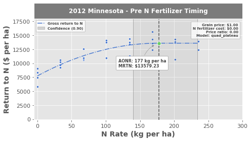
We see that the agronomic optimum nitrogen rate was calculated as 177 kg per ha, and the MRTN is 13.579 Mg per ha (yes, it says $13,579, but because price_grain was set to \$1, the values are equivalent and the units can be substituted.
If you’ve gone through the first tutorial, you’ll notice there are a few major differences in the look of this plot:
The red line representing nitrogen fertilizer cost is missing
The GRTN line does not pass through the y-intercept at \(\text{y}=0\)?
Because base_zero was set to False, the observed data (blue points) were not standardized as to “force” the best-fit model from passing through at \(\text{y}=0\).
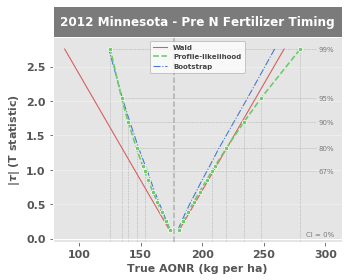
3.9. Bootstrap confidence intervals
We will calculate the AONR again, but this time we will compute the bootstrap confidence intervals in addition to the profile-likelihood and Wald-type confidence intervals. To tell EONR to compute the bootstrap confidence intervals, simply set bootstrap_ci to True in the EONR.calcualte_eonr() function:
[7]:
my_eonr.calculate_eonr(df_data, bootstrap_ci=True)
my_eonr.plot_tau()
my_eonr.fig_tau = my_eonr.plot_modify_size(fig=my_eonr.fig_tau.fig, plotsize_x=5, plotsize_y=4.0)
Computing AONR for Minnesota 2012 Pre
Cost of N fertilizer: $0.00 per kg
Price grain: $1.00 per kg
Fixed costs: $0.00 per ha
Agronomic optimum N rate (AONR): 177.4 kg per ha [139.9, 234.0] (90.0% confidence)
Maximum return to N (MRTN): $13579.23 per ha
3.10. Set fixed costs
Fixed costs (on a per area basis) can be considered by EONR. Simply set the fixed costs (using EONR.update_econ()) before calculating the EONR:
[8]:
costs_fixed = 12.00  # set to $12 per hectare
my_eonr.update_econ(costs_fixed=costs_fixed)
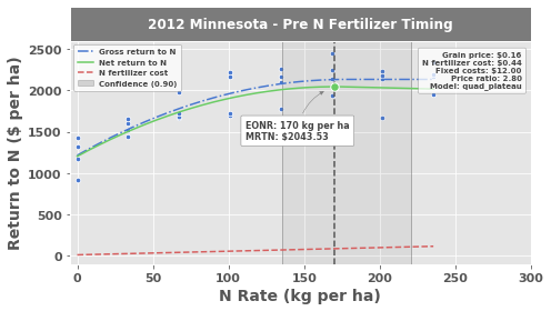
3.11. Loop through several economic conditions
EONR computes the optimum nitrogen rate for any economic scenario that we define. The EONR class is designed so the economic conditions can be adjusted, calculating the optimum nitrogen rate after each adjustment. We just have to set up a simple loop to update the economic scenario (using EONR.update_econ()) and calculate the EONR (using EONR.calculate_eonr()).
We will also generate plots and save them to our base directory right away:
[9]:
price_grain = 0.157  # set from $1 to 15.7 cents per kg
cost_n_fert_list = [0.44, 1.32, 2.20]

for cost_n_fert in cost_n_fert_list:
    # first, update fertilizer cost
    my_eonr.update_econ(cost_n_fert=cost_n_fert,
                        price_grain=price_grain)
    # second, calculate EONR
    my_eonr.calculate_eonr(df_data)
    # third, generate (and save) the plots
    my_eonr.plot_eonr(x_min=-5, x_max=300, y_min=-100, y_max=2600)
    my_eonr.plot_save(fname='eonr_mn2012_pre.png', fig=my_eonr.fig_eonr)
Computing EONR for Minnesota 2012 Pre
Cost of N fertilizer: $0.44 per kg
Price grain: $0.16 per kg
Fixed costs: $12.00 per ha
Economic optimum N rate (EONR): 169.9 kg per ha [135.2, 220.9] (90.0% confidence)
Maximum return to N (MRTN): $2043.53 per ha
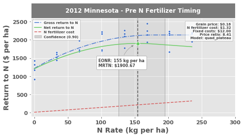
Computing EONR for Minnesota 2012 Pre
Cost of N fertilizer: $1.32 per kg
Price grain: $0.16 per kg
Fixed costs: $12.00 per ha
Economic optimum N rate (EONR): 154.8 kg per ha [125.7, 195.0] (90.0% confidence)
Maximum return to N (MRTN): $1900.67 per ha
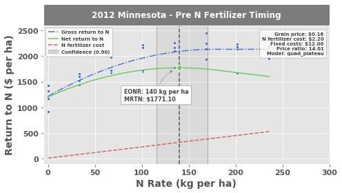
Computing EONR for Minnesota 2012 Pre
Cost of N fertilizer: $2.20 per kg
Price grain: $0.16 per kg
Fixed costs: $12.00 per ha
Economic optimum N rate (EONR): 139.7 kg per ha [115.9, 170.1] (90.0% confidence)
Maximum return to N (MRTN): $1771.10 per ha
A similar loop can be made adjusting the social cost of nitrogen. my_eonr.base_zero is set to True to compare the graphs:
[10]:
price_grain = 0.157  # keep at 15.7 cents per kg
cost_n_fert = 0.88  # set to be constant
my_eonr.update_econ(price_grain=price_grain,
                    cost_n_fert=cost_n_fert)
my_eonr.base_zero = True  # let's use base zero to compare graphs

cost_n_social_list = [0.44, 1.32, 2.20, 4.40]

for cost_n_social in cost_n_social_list:
    # first, update social cost
    my_eonr.update_econ(cost_n_social=cost_n_social)
    # second, calculate EONR
    my_eonr.calculate_eonr(df_data)
    # third, generate (and save) the plots
    my_eonr.plot_eonr(x_min=-5, x_max=300, y_min=-400, y_max=1400)
    my_eonr.plot_save(fname='eonr_mn2012_pre.png', fig=my_eonr.fig_eonr)
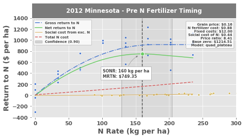
Computing SONR for Minnesota 2012 Pre
Cost of N fertilizer: $0.88 per kg
Price grain: $0.16 per kg
Fixed costs: $12.00 per ha
Social cost of N: $0.44 per kg
Socially optimum N rate (SONR): 160.1 kg per ha [129.0, 204.0] (90.0% confidence)
Maximum return to N (MRTN): $749.35 per ha
Computing SONR for Minnesota 2012 Pre
Cost of N fertilizer: $0.88 per kg
Price grain: $0.16 per kg
Fixed costs: $12.00 per ha
Social cost of N: $1.32 per kg
Socially optimum N rate (SONR): 155.8 kg per ha [126.3, 196.7] (90.0% confidence)
Maximum return to N (MRTN): $737.04 per ha
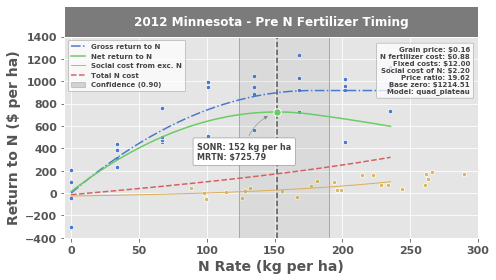
Computing SONR for Minnesota 2012 Pre
Cost of N fertilizer: $0.88 per kg
Price grain: $0.16 per kg
Fixed costs: $12.00 per ha
Social cost of N: $2.20 per kg
Socially optimum N rate (SONR): 151.8 kg per ha [123.8, 189.9] (90.0% confidence)
Maximum return to N (MRTN): $725.79 per ha
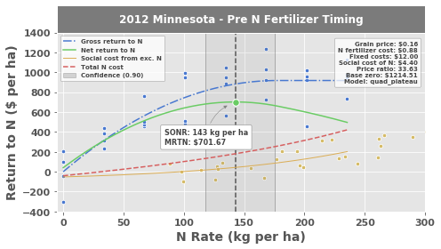
Computing SONR for Minnesota 2012 Pre
Cost of N fertilizer: $0.88 per kg
Price grain: $0.16 per kg
Fixed costs: $12.00 per ha
Social cost of N: $4.40 per kg
Socially optimum N rate (SONR): 142.8 kg per ha [117.9, 175.0] (90.0% confidence)
Maximum return to N (MRTN): $701.67 per ha

Notice that we used the same EONR instance (my_eonr) for all runs. This is convenient if there are many combinations of economic scenarios (or many experimental datasets) that you’d like to loop through. If you’d like the results to be saved separate (perhaps to separate results depending if a social cost is considered) that’s fine too. Simply create a new instance of EONR and customize how you’d like.
3.12. View results
All eight runs can be viewed in the dataframe:
[11]:
my_eonr.df_results
[11]:
| price_grain | cost_n_fert | cost_n_social | costs_fixed | price_ratio | unit_price_grain | unit_cost_n | location | year | time_n | ... | mrtn | grtn_r2_adj | grtn_rmse | grtn_max_y | grtn_crit_x | grtn_y_int | scn_lin_r2 | scn_lin_rmse | scn_exp_r2 | scn_exp_rmse | |
|---|---|---|---|---|---|---|---|---|---|---|---|---|---|---|---|---|---|---|---|---|---|
| 0 | 1.000 | 0 | 0.00 | 0 | 0.000000 | $ per ha | $ per kg | Minnesota | 2012 | Pre | ... | 13579.232456 | 0.728926 | 1154.305686 | 13579.232456 | 177.437339 | 7735.725352 | None | None | None | None |
| 1 | 1.000 | 0 | 0.00 | 0 | 0.000000 | $ per ha | $ per kg | Minnesota | 2012 | Pre | ... | 13579.232456 | 0.728926 | 1154.305686 | 13579.232456 | 177.437339 | 7735.725352 | None | None | None | None |
| 2 | 0.157 | 0.44 | 0.00 | 12 | 2.802548 | $ per ha | $ per kg | Minnesota | 2012 | Pre | ... | 2043.528038 | 0.728926 | 181.225993 | 2131.939496 | 177.437340 | 1214.508882 | None | None | None | None |
| 3 | 0.157 | 1.32 | 0.00 | 12 | 8.407643 | $ per ha | $ per kg | Minnesota | 2012 | Pre | ... | 1900.670950 | 0.728926 | 181.225993 | 2131.939496 | 177.437340 | 1214.508882 | None | None | None | None |
| 4 | 0.157 | 2.2 | 0.00 | 12 | 14.012739 | $ per ha | $ per kg | Minnesota | 2012 | Pre | ... | 1771.101634 | 0.728926 | 181.225993 | 2131.939496 | 177.437340 | 1214.508882 | None | None | None | None |
| 5 | 0.157 | 0.88 | 0.44 | 12 | 8.407643 | $ per ha | $ per kg | Minnesota | 2012 | Pre | ... | 749.347111 | 0.728926 | 181.225993 | 917.433580 | 177.439985 | 0.002964 | 0.777106 | 55.7255 | 0.836099 | 8.44737 |
| 6 | 0.157 | 0.88 | 1.32 | 12 | 14.012739 | $ per ha | $ per kg | Minnesota | 2012 | Pre | ... | 737.042610 | 0.728926 | 181.225993 | 917.433580 | 177.439985 | 0.002964 | 0.777106 | 167.176 | 0.836099 | 25.3421 |
| 7 | 0.157 | 0.88 | 2.20 | 12 | 19.617834 | $ per ha | $ per kg | Minnesota | 2012 | Pre | ... | 725.792236 | 0.728926 | 181.225993 | 917.433580 | 177.439985 | 0.002964 | 0.777106 | 278.627 | 0.836099 | 42.2368 |
| 8 | 0.157 | 0.88 | 4.40 | 12 | 33.630573 | $ per ha | $ per kg | Minnesota | 2012 | Pre | ... | 701.669696 | 0.728926 | 181.225993 | 917.433580 | 177.439985 | 0.002964 | 0.777106 | 557.255 | 0.836099 | 84.4737 |
9 rows × 33 columns
EONR.df_results contains the following data columns (some columns are hidden by Jupyter in the table above):
price_grain – price of grain
cost_n_fert – cost of nitrogen fertilizer
cost_n_social – other “social” costs of nitrogen
price_ratio – cost:grain price ratio
unit_price_grain – units descirbing the price of grain
unit_cost_n – units describing cost of nitrogen (both fertilizer and social costs)
location – location of dataset
year – year of dataset
time_n – nitrogen application timing of dataset
model – the model used to fit the experimental data (e.g., “quadratic” or “quad_plateau”).
base_zero – if
base_zero = True, this is the y-intercept (\(\beta_0\)) of the quadratic-plateau model before standardizing the dataeonr – optimum nitrogen rate (can be agronomic, economic, or socially optimum; in units of
EONR.unit_nrate)eonr_bias – bias in reparameterized quadratic-plateau model for computation of confidence intervals
R* – the coefficient representing the generalized cost function
costs_at_onr – total costs at the optimum nitrogen rate
ci_level – confidence interval (CI) level (for subsequent confidence bounds)
ci_wald_l – lower Wald CI
ci_wald_u – upper Wald CI
ci_pl_l – lower profile-likelihood CI
ci_pl_u – upper profile-likelihood CI
ci_boot_l – lower bootstrap CI
ci_boot_u – upper bootstrap CI
mrtn – maximum return to nitrogen (in units of
EONR.unit_currency)grtn_r2_adj – adjusted \(\text{r}^2\) value of the gross return to nitrogen (GRTN) model
grtn_rmse – root mean squared error of the GRTN
grtn_max_y – maximum y value of the GRTN (in units of
EONR.unit_rtn)grtn_crit_x – critical x-value of the GRTN (point where the “quadratic” part of the quadratic-plateau model terminates and the “plateau” commences)
grtn_y_int – y-intercept (\(\beta_0\)) of the GRTN model
scn_lin_r2 – adjusted \(\text{r}^2\) value of the linear best-fit for social cost of nitrogen
scn_lin_rmse – root mean squared error of the the linear best-fit for social cost of nitrogen
scn_exp_r2 – adjusted \(\text{r}^2\) value value of the exponential best-fit for social cost of nitrogen
scn_exp_rmse – root mean squared error of the the exponential best-fit for social cost of nitrogen
3.13. Save the data
The results generated by EONR can be saved to the EONR.base_dir using the Pandas df.to_csv() function. A folder will be created in the base_dir whose name is determined by the current economic scenario of my_eonr (in this case “social_336_4400”, corresponding to cost_n_social > 0, price_ratio == 33.6, and cost_n_social == 4.40 for “social”, “336”, and “4400” in the folder name, respectively):
[12]:
print(my_eonr.base_dir)

my_eonr.df_results.to_csv(os.path.join(os.path.split(my_eonr.base_dir)[0], 'advanced_tutorial_results.csv'), index=False)
my_eonr.df_ci.to_csv(os.path.join(os.path.split(my_eonr.base_dir)[0], 'advanced_tutorial_ci.csv'), index=False)
F:\nigo0024\Documents\GitHub\eonr\eonr\examples\eonr_advanced_tutorial\social_336_4400